By Ishan Shah

What is cross validation in machine learning?

Cross validation in machine learning is a technique that provides an accurate measure of the performance of a machine learning model. This performance will be closer to what you can expect when the model is used on a future unseen dataset.

The application of the machine learning models is to learn from the existing data and use that knowledge to predict future unseen events. The cross validation in machine learning model needs to be thoroughly done to profitably trade in live trading.

After reading this, you will be able to:

Determine if the machine learning model is good in predicting buy signal and/or sell signal
Demonstrate the performance of your machine learning trading model in different stress scenarios
Comprehensively do the cross validation in machine learning trading model

But before I explain how to do cross validation in machine learning model, I will first create a sample machine learning decision tree classifier model using price data of the Apple stock. Then, I'll implement various cross validation measures on this model. To implement this in Python, I'll follow the below steps

Importing the necessary libraries
Fetching the data
Defining the input and output dataset
Training the machine learning model

If you are already well versed with these steps and Python coding then you can skim through this part.

Importing the libraries

In [1]:

import quantrautil as q
import numpy as np
from sklearn import tree

The libraries imported above will be used as follows:

quantrautil - this will be used to fetch the price data of the AAPL stock from yahoo finance.
numpy - to perform the data manipulation on AAPL stock price to compute the input features and output. If you want to read more about numpy then it can be found here.
tree from sklearn - Sklearn has a lot of tools and implementation of machine learning models. 'tree' will be used to create Decision Tree classifier model.

Fetching the data

The next step is to import the price data of AAPL stock from quantrautil. The get_data function from quantrautil is used to get the AAPL data for 19 years from 1 Jan 2000 to 31 Dec 2018 as shown below. The data is stored in the dataframe aapl.

In [2]:

aapl = q.get_data('aapl','2000-1-1','2019-1-1')
print(aapl.tail())

[*********************100%***********************]  1 of 1 downloaded
                  Open        High         Low       Close   Adj Close  \
Date                                                                     
2018-12-24  148.149994  151.550003  146.589996  146.830002  146.830002   
2018-12-26  148.300003  157.229996  146.720001  157.169998  157.169998   
2018-12-27  155.839996  156.770004  150.070007  156.149994  156.149994   
2018-12-28  157.500000  158.520004  154.550003  156.229996  156.229996   
2018-12-31  158.529999  159.360001  156.479996  157.740005  157.740005   


Date         Volume         
2018-12-24  37169200  
2018-12-26  58582500  
2018-12-27  53117100  
2018-12-28  42291400  
2018-12-31  35003500

Creating input and output dataset

In this step, I will create the input and output variable.

Input variable: I have used '(Open-Close)/Open', '(High - Low)/Low', standard deviation of last 5 days returns (std_5), and average of last 5 days returns (ret_5)
Output variable: If tomorrow’s close price is greater than today's close price then the output variable is set to 1 and otherwise set to -1. 1 indicates to buy the stock and -1 indicates to sell the stock.

The choice of these features as input and output is completely random. If you are interested to learn more about feature selection, then you can read here.

In [3]:

# Features construction 
aapl['Open-Close'] = (aapl.Open - aapl.Close)/aapl.Open
aapl['High-Low'] = (aapl.High - aapl.Low)/aapl.Low
aapl['percent_change'] = aapl['Adj Close'].pct_change()
aapl['std_5'] = aapl['percent_change'].rolling(5).std()
aapl['ret_5'] = aapl['percent_change'].rolling(5).mean()
aapl.dropna(inplace=True)

# X is the input variable
X = aapl[['Open-Close', 'High-Low', 'std_5', 'ret_5']]

# Y is the target or output variable
y = np.where(aapl['Adj Close'].shift(-1) > aapl['Adj Close'], 1, -1)

Training the machine learning model

All set with the data! Let's train a decision tree classifier model. The DecisionTreeClassifier function from tree is stored in variable ‘clf’ and then a fit method is called on it with ‘X’ and ‘y’ dataset as the parameters so that the classifier model can learn the relationship between X and y.

In [4]:

clf = tree.DecisionTreeClassifier(random_state=5)
model = clf.fit(X, y)

The model is ready. But how do we do cross validation of this model? Here's how.

Cross validation of the machine learning model

If the cross validation is done on the same data from which the model learned then it is a no brainer that the performance of the model is bound to be spectacular.

In [5]:

from sklearn.metrics import accuracy_score
print('Correct Prediction: ', accuracy_score(y, model.predict(X), normalize=False))
print('Total Prediction: ', X.shape[0])

Correct Prediction:  4775
Total Prediction:  4775

As you can see above, all the predictions are correct. But there is a lot of Python code here. Yes! accuracy_score is a function from sklearn.metrics package which tells you how many predictions are correct. It takes as input the actual output (y) and predicted output (model.predict(X)), compares both the inputs and tells us how many of them were correct. If you want to see the output in percentage then set the normalized parameter to True as done below.

In [6]:

print(accuracy_score(y, model.predict(X), normalize=True)*100)

100.0

How do you overcome this problem of using the same data for training and testing?

One of the easiest and most widely used ways is to partition the data into two parts where one part of the data (training dataset) is used to train the model and the other part of the data (testing dataset) is used to test the model.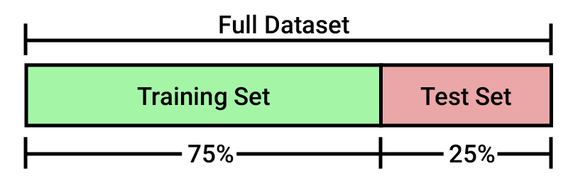 Cross Validation In Machine Learning 1

In [7]:

# Total dataset length
dataset_length = aapl.shape[0]

# Training dataset length
split = int(dataset_length * 0.75)
split

Out[7]:

In [8]:

# Splittiing the X and y into train and test datasets
X_train, X_test = X[:split], X[split:]
y_train, y_test = y[:split], y[split:]

# Print the size of the train and test dataset
print(X_train.shape, X_test.shape)
print(y_train.shape, y_test.shape)

(3581, 4) (1194, 4)
(3581,) (1194,)

In the above code, the total dataset of 4775 points is divided into two parts; first 75% of dataset creates X_train and y_train which contains the dataset to train the model and the remaining 25% of dataset creates X_test and y_test which contains the dataset to test the model. The choice of 75% is random.

In [9]:

# Create the model on train dataset
model = clf.fit(X_train, y_train)

In [10]:

# Calculate the accuracy
accuracy_score(y_test, model.predict(X_test), normalize=True)*100

Out[10]:

49.413735343383586

If you test the model on test dataset then a significant drop in accuracy is seen from 100% to 49.41%. The model performance in test dataset is closer to what you can expect if you take this model for live trading. However, there is still a major problem. The cross validation in the model is done on a single test dataset. In this example, on last 1194 data points. It could be by sheer luck that this model was able to predict with 49.41% in the test dataset. If I change the length of the train-test split from 75% to 80% or use different data points say first 1194 data points, then the accuracy of the model can vary a lot. Therefore, there is a need to test on multiple unseen datasets. But how do you achieve this?

K-Fold Cross Validation Technique

Don’t worry! K-fold cross validation technique, one of the most popular methods helps to overcome these problems. This method splits your dataset into K equal or close-to-equal parts. Each of these parts is called a "fold". For example, you can divide your dataset into 4 equal parts namely P1, P2, P3, P4. The first model M1 is trained on P2, P3, and P4 and tested on P1. The second model is trained on P1, P3, and P4 and tested on P2 and so on. In other words, the model i is trained on the union of all subsets except the ith. The performance of the model i is tested on the ith part. When this process is completed, you will end up with four accuracy values, one for each model. Then you can compute the mean and standard deviation of all the accuracy scores and use it to get an idea of how accurate you can expect the model to be. Cross Validation In Machine Learning 2

Some questions that you might have.

How do you select the number of folds?

The choice of the number of folds must allow the size of each validation partition to be large enough to provide a fair estimate of the model’s performance on it and shouldn’t be too small, say 2, such that we don’t have enough trained models to perform cross validation.

Why is this better than the original method of a single train and test split?

Well, as discussed above that by choosing a different length for the train and the test data split, the model performance can vary quite a bit, depending on the specific data points that happen to end up in the training or testing dataset. This method gives a more stable estimate of how the model is likely to perform on average, instead of relying completely on a single model trained using a single training dataset.

How can you perform cross validation of the model on a dataset which is prior to the dataset used to train the model? Is it not historically accurate?

If you train the model on a data from January 2010 to December 2018 and test on data from January 2008 to December 2009. Rightly so, the performance which we will obtain from the model will not be historically accurate. One of the limitations of this method. However, from the other side, this method can help to perform cross validation of how the model would have performed in the stress scenarios such as 2008. For example, when investors ask how the model would perform if stress scenarios such as the dot com bubble, housing bubble, or qe tapering occur again. Then, you can show the out-of-sample results of the model when such scenarios occurred. That should be likely performance when such scenarios occur again.

Code K-fold in Python

To code, KFold function from sklearn.model_selection package is used. You need to pass the number of splits required and whether to shuffle (True) the data points or not (False) to shuffle it and store it in a variable say kf. Then, call split function on kf and X as the input. The split function splits the index of the X and returns an iterator object. The iterator object is iterated using for loop and the integer index of train and test is printed.

In [11]:

from sklearn.model_selection import KFold
kf = KFold(n_splits=4,shuffle=False)

In [12]:

kf.split(X)

Out[12]:

<generator object _BaseKFold.split at 0x0000000009936F68>

In [13]:

print("Train: ", "TEST:")
for train_index, test_index in kf.split(X):
     print(train_index, test_index)

Train:  TEST:
[1194 1195 1196 ... 4772 4773 4774] [   0    1    2 ... 1191 1192 1193]
[   0    1    2 ... 4772 4773 4774] [1194 1195 1196 ... 2385 2386 2387]
[   0    1    2 ... 4772 4773 4774] [2388 2389 2390 ... 3579 3580 3581]
[   0    1    2 ... 3579 3580 3581] [3582 3583 3584 ... 4772 4773 4774]

The total dataset of 4775 points is divided into four different ways. For the first fold, points 0 to 1193 are used as test dataset and the points 1194 to 4774 are used as train dataset and so on. I'll create four different models for each of the fold shown above and determine the accuracy for each of the models. Again, this will be done through a for loop, by calling the fit method to train the model and by calling accuracy_score to determine the accuracy of the model.

In [14]:

# Initialize the accuracy of the models to blank list. The accuracy of each model will be appended to this list
accuracy_model = []

# Iterate over each train-test split
for train_index, test_index in kf.split(X):
    # Split train-test
    X_train, X_test = X.iloc[train_index], X.iloc[test_index]
    y_train, y_test = y[train_index], y[test_index]
    # Train the model
    model = clf.fit(X_train, y_train)
    # Append to accuracy_model the accuracy of the model
    accuracy_model.append(accuracy_score(y_test, model.predict(X_test), normalize=True)*100)# Print the accuracy    
print(accuracy_model)

[50.502512562814076, 49.413735343383586, 51.75879396984925, 49.79044425817267]

Stability of the model

Let's determine the variation and average accuracy of the model by calling the standard deviation and mean function from the numpy package.

In [15]:

np.std(accuracy_model)

Out[15]:

0.8939494614206329

In [16]:

np.mean(accuracy_model)

Out[16]:

50.3663715335549

The accuracy of the model is 50.36% +/- 0.89%. This is more likely to be the behaviour of the model in live trading.

Confusion Matrix

With the above accuracy, you got an idea about the accuracy of the model. But what is the model's accuracy in predicting each label such as Buy and Sell? This can be determined by using the confusion matrix. In the above example, the confusion matrix will tell you the number of times the actual value was 'buy' and predicted was also 'buy', actual value was 'buy' but predicted was 'sell' and so on.

In [18]:

# Import the pandas for creating a dataframe
import pandas as pd

# To calculate the confusion matrix
from sklearn.metrics import confusion_matrix

# To plot
%matplotlib inline
import matplotlib.pyplot as plt
import seaborn as sn

# Initialize the array to zero which will store the confusion matrix
array = [[0,0],[0,0]]

# For each train-test split: train, predict and compute the confusion matrix
for train_index, test_index in kf.split(X):
    # Train test split
    X_train, X_test = X.iloc[train_index], X.iloc[test_index]
    y_train, y_test = y[train_index], y[test_index]
    # Train the model
    model = clf.fit(X_train, y_train)
    # Calculate the confusion matrix
    c = confusion_matrix(y_test, model.predict(X_test))
    # Add the score to the previous confusion matrix of previous model
    array = array + c
# Create a pandas dataframe that stores the output of confusion matrix        
df = pd.DataFrame(array, index = ['Buy', 'Sell'], columns = ['Buy', 'Sell'])

# Plot the heatmap
sn.heatmap(df, annot=True, cmap='Greens', fmt='g')
plt.xlabel('Predicted')
plt.ylabel('Actual')
plt.show()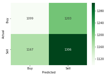

From the above confusion matrix, if you focus on the darker green zone (1306), that is when actual value was sell and model also predicted sell. Then, out of 2509 (1306+1203) times, the model was right 1306 times when it predicted the sell signal. That is an accuracy of 52%. From this, we can infer that the model is better in predicting the sell signal compared to the buy signal. Time to say goodbye! I hope you enjoyed reading this blog. Do share your feedback, comments, and request for the blogs. Cross validation in machine learning is an important tool in the trader's handbook as it helps the trader to know the effectiveness of their strategies. Now that you know the methodology of cross validation, you should check the course on Artificial Intelligence and test the effectiveness of the models.

Disclaimer: All data and information provided in this article are for informational purposes only. QuantInsti® makes no representations as to accuracy, completeness, currentness, suitability, or validity of any information in this article and will not be liable for any errors, omissions, or delays in this information or any losses, injuries, or damages arising from its display or use. All information is provided on an as-is basis. Suggested read: Working Of Neural Networks For Stock Price Prediction

Advanced Momentum Trading: Machine Learning Strategies Course